Chapter 04GQL by Example
This chapter introduces GQL through a concrete, self-contained library domain that we use as a running example throughout the book. Starting from an informal picture of the schema and a small instance, we show how to express the same structure using GQL’s data definition and manipulation features. We then formulate a series of queries over this graph, illustrating the core ideas of pattern matching, paths, and aggregation in the language.
4.1 Visual Representation
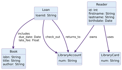
Figure 4.1 presents the schema as a type-level property graph, abstracting away from individual borrowers and concrete books to reveal the structural backbone of the library domain. Each rectangular box denotes a node type, specifying which attributes are available for entities of that kind. The Loan type, for example, states that every loan node must carry at least one identifying property, loanid: String, which uniquely characterizes a loan within the system. The LibraryAccount type introduces an analogous identifier num: String, representing the account code under which borrowings are recorded. The Reader type is richer: it combines a numeric identifier id: Int with textual attributes firstname: String and lastname: String, together with a birthdate: Date that captures the temporal dimension of the patron’s identity. A separate LibraryCard type models the physical card used at the circulation desk and self-service terminals; it has a single property num: String describing the card number printed on the plastic. Finally, the Book type specifies three bibliographic properties, isbn: String, title: String, and author: String, which together determine how book entities are represented in the graph.
The schema also defines its edge types and their property type sets. Edge type specifications carrying the labels owns, uses, check_out, and returns_to define typed connections between the corresponding node types: a Reader may own a LibraryAccount; the same Reader may use a LibraryCard; and a Loan is associated with a LibraryAccount via operations that record checking items out and returning them. Particularly noteworthy is the directed edge type from Loan to Book whose edge type label set is :INCLUDES. Unlike the other edge types, it declares the property types due_date: Date and late_fee: Float. This makes explicit that due dates and late fees are not inherent attributes of loans or books in isolation, but of the specific association between a given loan and a particular book instance. Taken together, the schema figure can be read as a compact contract for all valid library graphs in this model: it prescribes the node types that may exist, the edge types that may connect them, and the types of values that may decorate both nodes and relationships. The underlying property-graph structure and the formal definitions of node, edge, and graph types are given in Sections 6.2, 15.3 and 15.4.
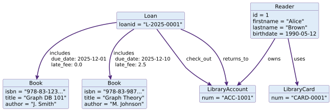
Figure 4.2 instantiates this schema with a small, concrete example of a library situation. At its center stands a single loan node, identified by the property loanid: “L-2025-0001”. This loan is tied to one library account node whose num: “ACC-1001” indicates the account under which the borrowing is registered. The account belongs to a specific reader, represented by a Reader node that carries basic personal data: an internal numeric identifier (id: 1), the first name “Alice”, the last name “Brown”, and the date of birth 1990-05-12. A separate LibraryCard node, with num: “CARD-0001”, captures the physical card that Alice uses to interact with the library system.
Two distinct Book nodes complete the picture. Each represents a different catalog item, described by an ISBN, a title, and an author. One book has isbn: “978-83-123...”, title: “Graph DB 101”, and author: “J. Smith”. The other is recorded as isbn: “978-83-987...”, title: “Graph Theory”, and author: “M. Johnson”. The edges stitching these nodes together mirror the schema’s relationship types. An edge labeled owns connects the reader to the library account, expressing that this account is Alice Brown’s. A second edge labeled uses links the reader to the library card, indicating that this card is the one she presents at the library.
The lifecycle of the borrowing process is then captured via edges from the loan node to the account node, with labels such as check_out and returns_to distinguishing the act of borrowing from the act of returning. The association between the loan and the individual books is modeled by includes edges from the loan node to each of the two book nodes. In the example, these relationship instances carry their own properties: one includes edge has due_date: 2025-12-01 and late_fee: 0.0, indicating that no late fee is recorded for that item, while the other has due_date: 2025-12-10 and late_fee: 2.5, showing that a fee has accrued for that particular item. In this way, the instance diagram can be read as a concrete graph that conforms to the structural constraints of the schema: every node and edge has exactly the label sets and property sets prescribed in the first illustration, turning the abstract specification into a tangible example of a library encoded as a property graph. The formal representation of this instance as sets of nodes, edges, labels, properties, and endpoints is given in Section 6.2.
4.2 Data Definition Language
The Data Definition Language (DDL) of GQL allows us to turn the informal schema of Figure 4.1 into an explicit graph type that constrains all admissible library graphs. In this example, we introduce a single graph type libraryGraphType. Its body specifies the node types (with their labels and property types), the edge types (with their labels, direction, and any edge properties), and a set of key constraints that capture the intended identifiers for loans, accounts, readers, cards, and books.
CREATE GRAPH TYPE libraryGraphType
AS {
  /* Node types */
  (Loan :Loan { loanid STRING NOT NULL }),
  (LibraryAccount :LibraryAccount { num STRING NOT NULL }),
  (Reader :Reader { id INT NOT NULL, firstname STRING,
                    lastname STRING, birthdate DATE }),
  (LibraryCard :LibraryCard { num STRING NOT NULL }),
  (Book :Book { isbn STRING NOT NULL, title STRING, author STRING }),

  /* Edge types */
  (Reader)-[:OWNS]->(LibraryAccount),
  (Reader)-[:USES]->(LibraryCard),
  (Loan)-[:CHECK_OUT]->(LibraryAccount),
  (Loan)-[:RETURNS_TO]->(LibraryAccount),
  (Loan)-[:INCLUDES { due_date DATE, late_fee FLOAT }]->(Book),

  /* Key constraints */
  CONSTRAINT LoanHasKey
    FOR (l:Loan)
    REQUIRE (l.loanid) IS KEY,
  CONSTRAINT LibraryAccountHasKey
    FOR (a:LibraryAccount)
    REQUIRE (a.num) IS KEY,
  CONSTRAINT ReaderHasKey
    FOR (r:Reader)
    REQUIRE (r.id) IS KEY,
  CONSTRAINT LibraryCardHasKey
    FOR (c:LibraryCard)
    REQUIRE (c.num) IS KEY,
  CONSTRAINT BookHasKey
    FOR (b:Book)
    REQUIRE (b.isbn) IS KEY
}
The body of the CREATE GRAPH TYPE statement declares the node types, edge types, and constraints that constitute libraryGraphType. Each parenthesized declaration, such as (Reader :Reader { id INT NOT NULL, firstname STRING, ... }), defines a node type. The identifier Reader is a local node type alias, :Reader specifies its label set, and the declarations inside braces specify the available properties together with their value types.
Similarly, the declaration
defines a directed edge type from Loan nodes to Book nodes. The edge has the label INCLUDES and may carry the properties due_date and late_fee, whose values must have the types DATE and FLOAT, respectively.
The CONSTRAINT clauses declare key constraints for selected node types. In each constraint, the FOR clause identifies the node type to which the constraint applies and binds a variable to matching nodes. For example, FOR (l:Loan) applies the constraint to Loan nodes and binds them to the variable l. The corresponding REQUIRE (l.loanid) IS KEY clause declares the loanid property as the key of that node type.
Consequently, loanid is the key of Loan nodes, num is the key of LibraryAccount nodes, id is the key of Reader nodes, num is the key of LibraryCard nodes, and isbn is the key of Book nodes. Graphs constrained by libraryGraphType must satisfy these key constraints in addition to the declared node and edge type requirements. If a modification would violate an applicable constraint or the constraining graph type, the offending operation does not complete successfully. The formal treatment of graph types, graph-type creation, key constraints, and their enforcement is given in Sections 15.4, 15.6, 16.1 and 16.2.
The following statement creates an empty graph constrained by this graph type:
CREATE GRAPH libraryGraph TYPED libraryGraphType
4.3 Data Manipulation Language
The Data Manipulation Language (DML) of GQL comprises the data-modifying statements INSERT, SET, REMOVE, and DELETE, together with procedure calls that execute data-modifying procedures. Where the Data Definition Language fixes the shape of admissible graphs via graph types and constraints, the DML operates on a particular graph instance. The graph named libraryGraph created above has libraryGraphType as its constraining graph type. All data-modifying statements act on the current working graph, which is selected by a USE clause at the beginning of a linear data-modifying statement. The selection of the current working graph by USE is formalized in Section 17.2.
Populating the graph. The following focused linear data-modifying statement inserts exactly the nodes and edges shown in Figure 4.2 into libraryGraph. The INSERT statement contains a single insert graph pattern, written as a collection of insert path patterns that share element variables such as l, a, r, c, b1, and b2. Each element pattern specifies labels and an initial property set using a { property key : value } notation.
USE libraryGraph
INSERT
  (l:Loan { loanid: 'L-2025-0001' })-
  [:CHECK_OUT]->(a:LibraryAccount {
    num: 'ACC-1001'
  }),
  (l)-[:RETURNS_TO]->(a),
  (r:Reader {
    id: 1,
    firstname: 'Alice',
    lastname: 'Brown',
    birthdate: DATE '1990-05-12'
  })-[:OWNS]->(a),
  (r)-[:USES]->(c:LibraryCard {
    num: 'CARD-0001'
  }),
  (l)-[:INCLUDES { due_date: DATE '2025-12-01',
                   late_fee: 0.0 }]->(b1:Book {
    isbn:  '978-83-123...',
    title: 'Graph DB 101',
    author: 'J. Smith'
  }),
  (l)-[:INCLUDES { due_date: DATE '2025-12-10',
                  late_fee: 2.5 }]->(b2:Book {
    isbn:  '978-83-987...',
    title: 'Graph Theory',
    author: 'M. Johnson'
  })
The first pattern creates a loan node l with property loanid and connects it, via a CHECK_OUT edge, to a library account node a whose identifier is the account number ’ACC-1001’. The next two patterns introduce the reader node r and the library card c: r is labeled :Reader and initialized with the personal attributes from the instance figure, and is connected to a and c by OWNS and USES edges, respectively. The final two patterns create two distinct book nodes, b1 and b2, each labeled :Book and equipped with its bibliographic properties, and attach them to the loan via INCLUDES edges. The edge property maps inside the braces specify the due date and late fee for each item. Because the schema in Figure 4.1 is declared as a constraining graph type, the evaluation of this statement is required to produce a graph that still conforms to libraryGraphType: all inserted elements must respect the declared element types, labels, and property types. The applicable constraints are validated before the statement completes successfully. The typing and operational semantics of this insertion are given in Section 14.1.
Updating properties with SET. Once the graph contains data, the SET statement can be used to change properties or labels of existing nodes and edges. In a typical pattern, a MATCH statement first binds element variables to the graph elements of interest, and a following SET statement updates their properties. The two statements together form a single linear data-modifying statement over the same working graph.
USE libraryGraph
MATCH (l:Loan { loanid: 'L-2025-0001' })-[i:INCLUDES]->(b:Book)
WHERE b.isbn = '978-83-987...'
SET   i.late_fee = 0.0
Here MATCH selects the INCLUDES edge i connecting loan L-2025-0001 to the book with the second ISBN. The SET statement then assigns a new value to i.late_fee, clearing the fee for this particular item. Because late_fee is declared as a FLOAT property type of the edge type whose label set is :INCLUDES, the value 0.0 is type-correct, and the update is required to preserve graph-type conformance. The read-then-update behavior and write-set semantics of this operation are given in Section 14.4.
Deleting graph elements. Finally, the DELETE statement removes nodes and edges from the working graph. When used with the DETACH keyword it also removes all edges incident to a deleted node. The following example deletes the loan node L-2025-0001 and all of its incident edges, while leaving the reader, account, card, and book nodes intact:
USE libraryGraph
MATCH (l:Loan { loanid: 'L-2025-0001' })
DETACH DELETE l
The MATCH clause binds the variable l to the unique loan node with the given identifier. The subsequent DETACH DELETE removes that node together with every edge attached to it, including the CHECK_OUT, RETURNS_TO, and INCLUDES edges shown in Figure 4.2. As with insertion and updates, the semantics of DELETE require that the resulting graph conforms to its constraining graph type and that its applicable constraints are satisfied before the statement completes successfully. In this example, deleting l and its incident edges preserves the declared property types and key constraints. The formal distinction between plain deletion and DETACH DELETE, including the treatment of incident edges, is given in Sections 14.2 and 16.2.
Taken together, these examples show how GQL’s DML can construct, evolve, and clean up concrete library graphs, while the graph type libraryGraphType and its constraints continue to govern the shape and well-formedness of every admissible state.
4.4 Data Query Language
The Data Query Language (DQL) of GQL provides read-only statements for navigating, filtering, and aggregating the data stored in a working graph. Syntactically, the examples in this section are instances of linear query statements in the sense of ISO 39075: they start with an optional USE clause and then apply a sequence of query statements such as MATCH, LET, and FILTER, followed by a primitive result statement of the form RETURN … optionally combined with an ORDER BY and LIMIT clause. All queries below assume that the working graph is the graph libraryGraph constrained by the graph type libraryGraphType introduced earlier. Each query is evaluated independently on the initial instance in Figure 4.2; the illustrative SET and DELETE statements above are not applied to that instance. Unless an ORDER BY clause is present, the displayed row order in the result tables is not significant.
Simple Rigid Pattern. A simple rigid pattern is a fixed arrangement of node and edge patterns without any path quantifiers or alternation. Such a pattern describes a specific configuration—a small neighborhood—that queries attempt to match exactly. In the library example, we might want to retrieve all items whose due date precedes a chosen reference date, together with the reader who borrowed them and the account through which the loan was recorded:
USE libraryGraph
MATCH (r:Reader)-[:OWNS]->(a:LibraryAccount),
      (r)-[:USES]->(c:LibraryCard),
      (l:Loan)-[i:INCLUDES]->(b:Book),
      (l)-[:CHECK_OUT]->(a)
WHERE i.due_date < DATE '2025-12-31'
RETURN r.firstname AS firstname,
       r.lastname  AS lastname,
       b.title     AS title,
       i.due_date  AS due_date,
       i.late_fee  AS late_fee
Expected result for the instance in Figure 4.2:
| firstname | lastname | title | due_date | late_fee |
| Alice | Brown | Graph DB 101 | 2025-12-01 | 0.0 |
| Alice | Brown | Graph Theory | 2025-12-10 | 2.5 |
The MATCH statement here consists of a graph pattern with four path patterns, separated by commas, that all share variables. The reader r is connected to a library account a via an OWNS edge and to a library card c via a USES edge. A loan l is connected by CHECK_OUT to the same account a and INCLUDES a book b via an edge i. The WHERE clause of the graph pattern restricts attention to those INCLUDES edges whose due_date precedes the given calendar date. The RETURN clause then projects a binding table whose columns correspond to the reader’s name, the title of the borrowed book, and the due date and late fee carried as edge properties on i. Because the pattern does not contain any path quantifiers, each solution row corresponds exactly to one concrete instance of this rigid configuration in the graph. The formal definitions of graph patterns, matching, binding-table formation, and result projection are given in Sections 7.1, 7.4 to 7.6 and 12.3.
Simple rigid patterns can be enriched with intermediate derived values using LET and subsequently filtered with FILTER. The next query looks for loans that contain both of the two example books and computes the total late fee incurred across those two items:
USE libraryGraph
MATCH (l:Loan)-[i1:INCLUDES]->(b1:Book),
      (l)-[i2:INCLUDES]->(b2:Book)
WHERE b1.isbn = '978-83-123...'
  AND b2.isbn = '978-83-987...'
LET  total_late_fee = i1.late_fee + i2.late_fee
FILTER WHERE total_late_fee > 0.0
RETURN l.loanid       AS loanid,
       total_late_fee AS totalLateFee
Expected result for the instance in Figure 4.2:
| loanid | totalLateFee |
| L-2025-0001 | 2.5 |
The graph pattern selects pairs of INCLUDES edges i1 and i2 that originate from the same loan l but point to different books b1 and b2 with the specified ISBN values. The LET statement introduces a value variable total_late_fee computed by adding the two edge-local late fee amounts. The FILTER statement then retains only those bindings for which the derived total is strictly positive. Here, the WHERE clause is part of the graph pattern and restricts that pattern’s matches. By contrast, FILTER [WHERE] is a separate simple query statement that filters the current working table and can use bindings introduced by preceding statements, such as LET. The final RETURN projects the loan identifier and the computed totalLateFee, illustrating how rigid patterns, local arithmetic, and binding-table filters combine within a single linear query. The corresponding selection and projection operations, including the three-valued interpretation of filtering predicates, are formalized in Sections 8.3 and 9.1.
Conjunctive Regular Path Queries. Conjunctive Regular Path Queries (CRPQs) extend simple patterns by allowing conjunctions of multiple path patterns that share variables. In logical terms, a CRPQ describes several paths through the graph that must be simultaneously present and must meet joint constraints on shared endpoints or intermediate nodes. Even without explicit path quantifiers, the library domain already exhibits meaningful CRPQs.
Consider the task of finding pairs of readers who have, possibly at different times, borrowed the very same book. We are interested in such co-borrowers of the same book instance, but we want to list each unordered pair only once:
USE libraryGraph
MATCH (r1:Reader)-[:OWNS]->(a1:LibraryAccount),
      (r2:Reader)-[:OWNS]->(a2:LibraryAccount),
      (l1:Loan)-[:CHECK_OUT]->(a1),
      (l2:Loan)-[:CHECK_OUT]->(a2),
      (l1)-[:INCLUDES]->(b:Book),
      (l2)-[:INCLUDES]->(b)
WHERE r1.id < r2.id
RETURN DISTINCT r1.firstname AS reader1_firstname,
       r1.lastname  AS reader1_lastname,
       r2.firstname AS reader2_firstname,
       r2.lastname  AS reader2_lastname,
       b.title      AS common_title
Expected result for the instance in Figure 4.2:
| Result | Rows |
| Empty binding table | 0 |
This query consists of several path patterns that are conjoined by commas into a single graph pattern. Two readers r1 and r2 own accounts a1 and a2, respectively. Each account has at least one loan (l1 or l2) that checks out that account, and each of those loans includes the same book node b. The shared variable b enforces that the two paths meet at a common book, which is exactly the kind of join between paths that CRPQs support. The inequality predicate r1.id < r2.id in the WHERE clause removes the second ordering of each reader pair. RETURN DISTINCT also coalesces duplicate projected rows that can arise from multiple matching loans or parallel matches, so each projected reader-pair and title combination is reported once. The RETURN clause surfaces both readers’ names and the shared book title.
In full generality, regular path patterns in GQL can also use path quantifiers and alternation to describe arbitrarily long routes through the graph. The present example already illustrates the key idea of CRPQs: multiple path patterns, possibly of different lengths, are matched jointly, with constraints expressed over the shared nodes and edges. The joint matching of path-pattern components through shared variables is formalized in Sections 7.1 and 7.4.
Linear Composition. Linear composition refers to the way in which a GQL query can be built as a sequence of simple query statements that gradually transform the current working table. Each step—a MATCH, LET, or FILTER statement—takes the bindings produced so far, extends them with new variables, or discards those that fail a predicate. The final step is a primitive result statement that projects and optionally orders or pages the result.
The following query finds all books borrowed by a reader with the last name ’Brown’, restricts attention to items whose due date precedes a reference date, and orders the result by due date:
USE libraryGraph
MATCH (r:Reader)-[:OWNS]->(a:LibraryAccount)
WHERE r.lastname = 'Brown'
MATCH (a)<-[:CHECK_OUT]-(l:Loan)-[i:INCLUDES]->(b:Book)
FILTER WHERE i.due_date < DATE '2025-12-31'
RETURN l.loanid   AS loanid,
       b.title    AS title,
       i.due_date AS due_date,
       i.late_fee AS late_fee
ORDER BY due_date
Expected result for the instance in Figure 4.2:
| loanid | title | due_date | late_fee |
| L-2025-0001 | Graph DB 101 | 2025-12-01 | 0.0 |
| L-2025-0001 | Graph Theory | 2025-12-10 | 2.5 |
The first MATCH and its WHERE clause define the initial binding table: each row binds r and a to a reader with last name ’Brown’ and one of their accounts. The second MATCH uses these bindings as input and extends each row with a loan l, an INCLUDES edge i, and a book b that form the following fixed path:
(a)<-[:CHECK_OUT]-(l)-[:INCLUDES]->(b)
The FILTER statement then prunes those rows where i.due_date is not before the given reference date. Finally, the RETURN projects a smaller record—loan identifier, book title, due date, and late fee—and the trailing ORDER BY clause orders the resulting binding table by the due date column. This example shows how successive MATCH and FILTER statements can replace the kind of pipeline-oriented WITH clause found in other graph query languages, while remaining within the linear composition framework defined by the standard. The formal treatment of successive MATCH operations and whole-query pipeline composition is given in Sections 7.6, 9.5 and 12.3.
Order, Limit, and Aggregation. Aggregation, ordering, and pagination complete the picture by allowing queries to summarize larger result sets and to return just the most relevant rows. In GQL, aggregation is expressed via aggregate functions such as SUM and COUNT, and is combined with a GROUP BY clause inside the RETURN statement body. Ordering and limiting are provided by an ORDER BY and LIMIT clause, which together form the attached to the RETURN.
The next query computes, for each author, the total late fees incurred on loans of their books, and then returns the ten authors with the highest total late fee:
USE libraryGraph
MATCH (l:Loan)-[i:INCLUDES]->(b:Book)
LET   authorName = b.author
RETURN authorName           AS author,
       SUM(i.late_fee)      AS total_late_fee
GROUP BY author
ORDER BY total_late_fee DESC
LIMIT 10
Expected result for the instance in Figure 4.2:
| author | total_late_fee |
| M. Johnson | 2.5 |
| J. Smith | 0.0 |
The MATCH statement produces bindings of loans, INCLUDES edges, and books. The LET statement then introduces a value variable authorName that extracts the author property of each matched book. Inside the RETURN statement, the GROUP BY clause groups the current working table by the return-item alias author, and the aggregate function SUM(i.late_fee) computes, for each such group, the total amount of late fees associated with that author’s books. The two return items are projected under the aliases author and total_late_fee; these aliases become columns of the outgoing binding table. The trailing ORDER BY–LIMIT combination forms an order-by-and-page statement: it sorts the grouped rows in descending order of total_late_fee and retains only the first ten records. The overall linear query statement thus exemplifies how grouping, ordering, and pagination interact in a way that is faithful to the formal semantics of RETURN, GROUP BY, and the order-by-and-page statement in the GQL standard. The formal semantics of grouping, aggregate evaluation, result formation, ordering, and limiting is given in Sections 12.1, 12.3, 13.1 and 13.3.